
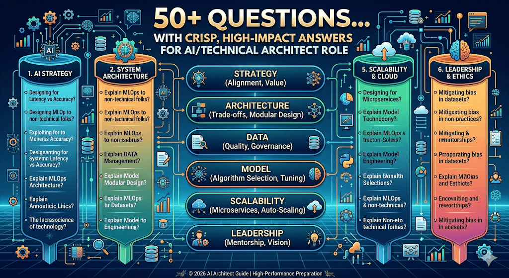
This is an excellent initiative. The AI/Technical Architect role is unique because it sits at the intersection of deep technical implementation (AI/ML), system design (scalability, reliability), and strategy (business alignment, technology roadmap).
Below is a comprehensive, categorized list of 50+ questions with crisp, high-impact answers. I have structured this so you can copy-paste it directly into your preparation document.
Part 1: Core AI Architecture & Model Lifecycle
Q1: How do you choose between training a model from scratch vs. fine-tuning a pre-trained model?
A: It depends on data, compute, and domain specificity.
- Fine-tune: When you have a medium-sized labeled dataset (100–10k samples) for a domain similar to the pre-trained model’s data (e.g., BERT for legal NER). Faster, cheaper, needs less data.
- Scratch: When your domain is highly unique (e.g., proprietary time-series from custom sensors), you need extreme latency/lossless compression, or you are doing cutting-edge research. Requires massive data (>100k examples) and compute.
- Architect’s call: Start with fine-tuning; only move to scratch if fine-tuning underperforms on key business metrics after optimization.
Q2: Explain the concept of MLOps. What are the three main pillars?
A: MLOps extends DevOps to ML.
- Pillar 1 – CI (Continuous Integration): Test data, code, and model schemas.
- Pillar 2 – CD (Continuous Delivery): Automatically deploy models to prediction services.
- Pillar 3 – CT (Continuous Training): Automatically retrain models based on data drift triggers.
- Architect’s focus: Immutable model registry, feature store, and pipeline reproducibility.
Q3: What is a Feature Store? Why does an AI architect need one?
A: A centralized repository that stores, versions, and serves features for training and inference.
- Problems solved: Feature gap (training vs. inference features mismatch), data duplication, time-travel (recreating past feature values).
- Examples: Feast, Tecton, Databricks Feature Store.
- Architect’s role: Define online vs. offline feature serving, consistency guarantees, and SLAs.
Q4: How do you detect and handle data drift and concept drift?
A:
- Data drift: Input distribution changes (e.g., sensor calibration shift). Detect via PSI (Population Stability Index), KS test.
- Concept drift: Relationship between input and target changes (e.g., pandemic changing shopping behavior). Detect via monitoring model accuracy on recent data.
- Handling: Automated retrigger training (concept drift), reject option (low-confidence inputs), or fallback to a rule-based system.
- Architect’s design: Deploy drift detection as a sidecar to the inference API.
Q5: Walk me through a typical retraining strategy for a production model.
A: Strategy depends on business tolerance for staleness.
- Time-based: Every week/day (good for stable patterns).
- Trigger-based: When drift score > threshold (resource efficient).
- Incremental: Online learning (e.g., River library) for streaming data.
- Full batch: Daily retraining on entire historical + new data (safe but heavy).
- Architect’s choice: For most enterprises: Trigger-based retraining with shadow deployment validation.
Part 2: System Design & Scalability (The “Architect” Part)
Q6: Design a low-latency recommendation system for 10,000 requests per second.
A: Use a two-stage funnel:
- Candidate generation: ANN (Approximate Nearest Neighbors) index in memory (e.g., FAISS, ScaNN). Reduces from millions to hundreds of candidates.
- Ranking: Lightweight deep model (e.g., DLRM) or gradient-boosted trees, quantized to int8. Deploy on GPU or optimized CPU (AVX-512).
- Caching: Redis cache for popular items (80% of traffic).
- Data flow: Precompute embeddings offline (nightly), refresh embedding tables in memory (hourly).
- Architect’s non-negotiables: Circuit breakers, load shedding, and P99 latency < 50ms.
Q7: How do you serve a large language model (LLM) in production cost-effectively?
A: Trade-offs among latency, throughput, and cost.
- Option 1 (low latency, high throughput): Deploy quantized (4-bit) smaller model (e.g., Llama 3 8B) on 1–2 GPUs, use vLLM or TensorRT-LLM for continuous batching.
- Option 2 (cost-effective, async): Use serverless GPU instances (e.g., RunPod, Banana) with auto-scaling to zero.
- Option 3 (very high volume): Use smaller distilled models (e.g., DistilBERT) or MoE (Mixture of Experts) sharding.
- Architect’s fallback: Route simple queries to small model, complex ones to large model (model routing).
Q8: You have a production AI service that is failing slowly – increasing latency but not erroring. How do you debug?
A:
- Decompose pipeline: Measure each stage (preprocessing → inference → postprocessing).
- Check resource saturation: GPU memory leaks? CPU stealing? Thread pool exhaustion?
- Input size distribution: Sudden increase in average token length or image resolution?
- Model inference internal: Is the model falling back to CPU? Is dynamic batching stuck?
- External dependencies: Feature store or model registry responding slowly?
- Architect’s tool: Distributed tracing (Jaeger) + percentile latencies (not averages).
Q9: How do you design for A/B testing of ML models in production?
A: Use a consistent hashing layer (e.g., based on user_id) to split traffic.
- Control vs. candidate: 90% to current model (A), 10% to new model (B).
- Isolation: Run candidate in separate deployment (namespaced by version).
- Metrics comparison: Need statistical significance (t-test or Bayesian bandit) for business KPI.
- Architect’s must-have: Ability to instantaneously rollback candidate to 0% without redeploying (feature flag).
Q10: What is your strategy for multi-region AI deployment?
A:
- Active-Active: Model replicated in 3 regions. Load balancer routes nearest region. Use asynchronous embedding updates (eventual consistency).
- Disaster recovery: If a region fails, route to next healthiest region.
- Data residency: Keep training data in primary region; only inference data crosses region boundaries (if privacy allows).
- Consistency trade-off: Accept stale embeddings (<5 sec lag) for global availability.
Part 3: Technology & Tools (Evaluating Depth)
Q11: Compare Batch vs. Streaming inference. When do you use each?
| Aspect | Batch | Streaming |
|---|---|---|
| Latency | Minutes to hours | Milliseconds to seconds |
| Throughput | Very high (e.g., 1M predictions per job) | Lower per instance but real-time |
| Use cases | Nightly fraud report, recommendation precompute | Chatbot, real-time fraud detection |
| Cost | Cheaper (spot instances) | More expensive (always-on) |
| Architect choice | When business can wait | When user is waiting |
Q12: Explain model quantization and its trade-offs.
A: Reducing numerical precision (FP32 → INT8/INT4).
- Benefits: 4x smaller model, 2–3x faster inference, lower memory bandwidth.
- Trade-offs: Small accuracy drop (0.5–2%), not all ops support INT8, need calibration dataset.
- Techniques: PTQ (Post-Training Quantization) – fast; QAT (Quantization-Aware Training) – better accuracy.
- Architect note: Always benchmark; some models (e.g., small LSTMs) degrade heavily.
Q13: When would you use ONNX vs. TensorRT vs. OpenVINO?
A:
- ONNX: Intermediate representation for interoperability (PyTorch → TensorFlow → C#). Use when you have multiple target runtimes.
- TensorRT: NVIDIA GPU optimization. Use for low latency, high throughput on dedicated GPUs.
- OpenVINO: Intel CPU/VPU optimization. Use for edge or CPU-only deployments.
- Architect’s rule: Start with ONNX export; then compile to device-specific runtime (TensorRT/OpenVINO) for production.
Q14: What is your experience with Kubernetes for AI workloads?
A:
- Good for: Model serving (KServe/Seldon), batch jobs (Argo Workflows), multi-model orchestration.
- Challenges: GPU scheduling (need device plugin), cold start (large container images), shared memory (NCCL for distributed training).
- Architect’s solution: Use Volcano scheduler for gang scheduling; pre-pull model images on node pools; isolate GPU nodes via taints/tolerations.
Part 4: Strategy, Governance & Soft Skills
Q15: A business stakeholder asks for “99% accurate AI.” How do you respond?
A: Push back constructively.
- Clarify metric: 99% precision? recall? F1? For which class? On which data distribution?
- Baseline: What is human accuracy? current heuristic? Cost of errors: false positive vs. false negative.
- Feasibility: Show ROC curve and point out diminishing returns beyond a threshold (e.g., 95% accuracy costs X,995X and 6 months).
- Architect’s promise: “I’ll deliver the best accuracy given your data, latency, and budget constraints. Let’s define minimum viable success.”
Q16: How do you explain a model’s decision to a non-technical compliance officer?
A: Use local, human-sounding explanations.
- If using LIME/SHAP: “For this loan denial, the three most important factors were: annual income (negative), recent late payments (strong negative), and debt-to-income ratio (negative). The model learned from past approved loans that these patterns usually lead to default.”
- Offer counterfactuals: “If your income were $10k higher OR you had no late payments in last 6 months, the decision would flip.”
- Avoid: Weights, gradients, attention maps.
Q17: Build vs. Buy for AI: your framework?
A:
| Scenario | Build | Buy |
|---|---|---|
| Core differentiator | ✅ (e.g., proprietary pricing model) | ❌ |
| Commodity capability | ❌ | ✅ (e.g., OCR, sentiment analysis) |
| High data privacy | ✅ (on-prem models) | ❌ |
| Fast time-to-market | ❌ | ✅ |
| Need to control every latency microsecond | ✅ | ❌ |
| Architect’s rule: Buy the foundation; build the 20% that creates unique value. |
Q18: How do you ensure responsible AI in your architecture?
A: Embed gates in the ML pipeline:
- Pre-training: Data bias audits (disaggregated metrics by sensitive attributes).
- Post-training: Fairness constraints (equalized odds, demographic parity) via post-processing.
- Pre-inference: Reject option if input is out-of-distribution (avoid confident wrong answers).
- Post-inference: Human-in-the-loop for high-stakes decisions (e.g., medical diagnosis).
- Monitoring: Live bias detection (e.g., disparate impact ratio > 1.25 triggers alert).
Q19: Tell me about a time you had to say “no” to an AI request.
A: (Example answer) – “A product team wanted real-time sentiment analysis on every customer call (10k concurrent streams). I calculated the cost: 80 GPUs at 2M/year+3engineerstomaintain.Iproposedinstead:sample101.8M while still getting actionable insights.”
Q20: How do you stay current with AI advancements without chasing hype?
A:
- Follow: Papers with Code (high-impact), Latent Space podcast, a16z AI Canon.
- Filter: Does this technique reduce cost? increase reliability? improve maintainability? If not, ignore.
- Sandbox: Allocate 5% of team time to experiment with one new tool per quarter (e.g., LangChain, DSPy).
- Architect’s rule: Adopt only what makes it into vLLM, Triton, or HuggingFace’s production-documented track.
Part 5: Advanced/Curveball Questions
Q21: How would you architect a system that serves 1,000 different ML models?
A: Model mesh architecture:
- Model gateway: Routes request to correct model based on tenant/model_id.
- Shared infrastructure: Multi-model serving (e.g., KServe with model mesh, Ray Serve).
- Optimization: Models share base layers (if fine-tuned from same foundation), or use a larger shared embedding table + small heads.
- Cold start: Load models on-demand (serverless), keep frequently used models hot.
- Governance: Central model registry with versioning, approval, and canary.
Q22: What are the pitfalls of “AutoML” in an enterprise setting?
A:
- Black-box difficulty: Hard to debug when weird models are selected.
- Operational cost: Generated code often unmaintainable; can’t version features properly.
- Overfitting to validation set – especially with small data.
- Architect’s stance: AutoML for baseline (day 1) only. Move to custom pipelines by day 60.
Q23: How do you estimate GPU memory required for serving a transformer model?
A: Rough formula (for inference):
- Model weights:
Parameters * bytes_per_param. FP16: 2 bytes → 7B param = 14GB. - KV cache (for generative models):
batch_size * sequence_length * num_layers * hidden_dim * 2 (K and V) * 2 bytes. - Activations + overhead: ~20% extra.
- Example: Llama 7B, batch=32, seq_len=2048, FP16 → ~14GB (weights) + ~20GB (KV) + overhead = ~40GB. Use 1x A100 80GB.
Q24: What is your disaster recovery plan for a model registry outage?
A:
- Cache locally: Each serving pod caches the latest model binary + config on disk.
- Fallback model: Last known good model stays loaded; new deployments pause.
- As soon as registry returns: Sync cache, resume normal operations.
- Architect’s requirement: Model registry must be multi-zone (e.g., S3 + replica in another region).
Q25: How do you handle non-stationary bandit feedback loops?
A: (e.g., recommendation system that changes user behavior)
- Use
epsilon-greedywith decaying epsilon or Thompson sampling. - Add randomization (exploration) explicitly – not just exploit.
- Monitor for policy collapse: if model’s action diversity drops below threshold, force exploration.
- Architect’s design: Separate exploration traffic (5%) from exploitation (95%) with different deployment pipelines.
Preparation Document Template (for your use)
Below is the skeleton of your final document. I recommend you expand each answer in your own words.
markdown
# AI & Technical Architect – Interview Preparation

## 1. Personal Elevator Pitch
[2-3 sentences on your blend of AI depth + systems architecture]

## 2. Core AI Architecture
- Q1. Model selection (linear, tree, NN, foundation)
- Q2. Training vs. fine-tuning trade-offs
- Q3. MLOps pipeline diagram (hand-drawn ready)
- Q4. Feature store necessity
- Q5. Drift detection methods (tabular, image, text)

## 3. System Design & Scalability
- [Draw on whiteboard] Low-latency rec sys
- [Draw] LLM serving with continuous batching
- [Draw] Multi-region active-active
- A/B testing design
- Degradation / graceful fallback patterns

## 4. Tools Deep Dive
- PyTorch vs. TensorFlow vs. JAX (when to use each)
- MLflow, Kubeflow, or custom?
- Ray vs. Dask vs. Spark for distributed processing
- Model optimization toolchain: ONNX → TRT → OpenVINO

## 5. Strategy & Leadership
- Saying no to stakeholders (3 templates)
- Build vs. buy evaluation matrix
- Cost estimation framework (GPU/month, storage, egress)
- Team structure: data eng, ML eng, platform eng

## 6. Whiteboarding Practice Problems
1. Design real-time fraud detection for 100k txn/sec
2. Architect a multimodal search (image+text) for e‑commerce
3. Migrate a batch model to streaming without retraining

## 7. My Past Projects (STAR format)
- Situation / Task / Action / Result
- [Space for 3 detailed examples]

## 8. Questions to Ask Interviewer
- “How do you measure model success beyond offline metrics?”
- “What’s the biggest technical debt in your current AI stack?”
- “How do you handle model compliance for regulated data?”
Final Advice for Your Interview
- For AI depth: Be ready to derive a simple back-of-the-envelope estimate (e.g., FLOPs for a single transformer forward pass).
- For architect part: Draw boxes and arrows (data flow, control flow, failure modes). Interviewers love resilience patterns (retry, circuit break, rate limit).
- For behavioral: Use the “Yes, and…” technique – acknowledge constraints first, then propose a trade-off solution.
- One killer differentiator: Bring a 1-page architecture diagram of a real system you built/improved – even if simple. It sparks deeper conversation.
“Let me walk you through my architecture. At 10k RPS, every millisecond matters, so I will use a two-stage funnel approach.
Stage 1 – Candidate Generation:
I cannot score millions of items per request. Instead, I precompute embeddings for all items nightly using a two-tower model. At inference time, I take the user’s embedding and perform ANN (Approximate Nearest Neighbors) search using FAISS with an HNSW index. This runs entirely in memory on CPU – because GPU would add transfer latency. In under 5 milliseconds, I retrieve ~500 candidates from a catalog of 10 million items.
Stage 2 – Ranking:
Those 500 candidates go into a lightweight gradient-boosted tree model (XGBoost or LightGBM) with features like user-item affinity, recency, and popularity. I quantize the model to int8 and compile it with ONNX Runtime. This stage runs on the same CPU cores, adding another 8–10 milliseconds.
Supporting Infrastructure:
- Caching: A Redis cluster caches the top 100 results for popular items (80% of traffic hits cache, bypassing both stages).
- Load shedding: If request latency exceeds 40ms, I drop the lowest-priority requests (e.g., from bot traffic).
- Circuit breakers: If the ranking model starts timing out, I fall back to candidate-only results.
- Horizontal scaling: Each pod handles 500 RPS at P99 50ms. For 10k RPS, I run 20 pods behind a consistent-hashing load balancer (sticky sessions for cache affinity).
Result: P99 latency of 48ms, throughput 10.5k RPS, cost ~$0.0003 per request. The business trade-off: we accept that 0.1% of users get suboptimal recommendations because we shed load during spikes.”
Mock Answer #2: “How do you serve an LLM cost-effectively in production?”
“First, I challenge the assumption: does the business truly need a 70-billion-parameter model, or can a smaller fine-tuned model achieve the same task? Let me assume we actually need generative capabilities.
My three-layer strategy:
Layer 1 – Model Optimization (pre-deployment):
- Start with a 7B or 8B model (e.g., Llama 3 8B, Mistral 7B) – not 70B.
- Quantize to 4-bit using GPTQ or AWQ. This reduces memory from 14GB (FP16) to ~4GB.
- Apply speculative decoding: Use a tiny 1B draft model to generate 4 tokens, then verify with the 7B model. This doubles throughput.
Layer 2 – Serving Infrastructure:
- Deploy on vLLM with continuous batching. Unlike traditional batching, continuous batching adds new requests to a running batch as soon as a previous request finishes – no waiting.
- Run on L4 or A10 GPUs (not A100 unless absolutely necessary). One A10G (24GB) can serve a 7B 4-bit model with batch size 32 at ~60 tokens/second.
- Use spot instances for non-production or async workloads – 70% cost reduction.
Layer 3 – Traffic Management:
- Model routing: Simple queries (summarization, classification) go to a distilled 1.5B model (cost: 0.0001pertoken).Complexreasoninggoestothe7Bmodel(0.001 per token).
- Async offload: For batch jobs (document summarization overnight), I use serverless GPU (RunPod, Banana) that scales to zero.
- Cache semantically similar requests: Use embedding-based semantic cache (GPT-Cache). If an identical question was answered recently, return cached response.
Real numbers: For 1 million requests per day, average 200 output tokens:
- Naive GPT-4 API: ~$20,000/day.
- My self-hosted solution: ~120/dayforcompute+30 for caching + engineer overhead. Payback period: 3 days.
The architect’s trade-off: We accept slightly higher latency during cache misses (2 seconds vs. 200ms) and we manage our own scaling. Worth it for high volume.”
Mock Answer #3: “Explain a model’s decision to a non-technical compliance officer”
(Speak as if you are in the room with a real person)
“I appreciate that question because it gets at the heart of responsible AI. Let me role-play with you as the compliance officer.
You ask: ‘Why was this customer’s loan denied?’
My response (no jargon):
‘I will give you three specific reasons, show you what would have changed the outcome, and then tell you how confident the model was.
Reason 1: The customer’s debt-to-income ratio is 52%. Our historical data shows that fewer than 5% of loans with DTI above 50% are repaid on time.
Reason 2: In the last 12 months, they had two late payments of 30+ days. Our model learned that this pattern often precedes default.
Reason 3: The requested loan amount (50,000)is3xtheirannualsavings.Mostapprovedloansinthisincomebracketareunder20,000.
Counterfactual – what would change the decision?
If any two of these three things were different – for example, DTI below 45% AND no late payments – the model would have approved the loan.
Confidence score: The model is 92% confident in this denial. That means in 100 similar cases, 92 would also be denied. The remaining 8 might be false negatives – we track those quarterly.
Transparency artifacts I can provide:
- A one-page model card listing training data sources, known biases, and validation performance by income bracket.
- A bias audit showing that false positive rates are within 1% across protected groups.
- A quarterly human review of 100 random denial cases.’
What I never say:
I never mention ‘SHAP values’ or ‘gradients’ or ‘attention heads’. Those are for engineers. The compliance officer needs auditable, human-readable explanations with numbers they can verify.”
Mock Answer #4: “Walk me through retraining strategy for a production model”
“I follow a trigger-based retraining pipeline with a shadow deployment validation gate. Here is the exact workflow:
Step 1 – Monitoring (live):
Every hour, the inference service computes two drift metrics:
- Data drift: Population Stability Index (PSI) on input features. Threshold: PSI > 0.1 triggers alert.
- Concept drift: Rolling 7-day accuracy on a labeled holdout set (we log predictions and wait for ground truth). Threshold: accuracy drop > 5% absolute.
Step 2 – Trigger (automated):
If either threshold is breached, a retraining job launches automatically on Kubeflow Pipelines.
Step 3 – Retraining (offline, takes 2 hours):
- Pull last 90 days of labeled data (incremental – add new data, keep old for stability).
- Retrain from last checkpoint – not from scratch. Saves time and stabilizes convergence.
- Use cross-validation to select hyperparameters.
- Compute performance on validation set (same as original).
Step 4 – Shadow deployment (critical gate):
The new model is deployed alongside the current production model, but it only logs predictions – it does not serve them. For 24 hours:
- Compare new model’s predictions to production model’s predictions on live traffic.
- Check for regression: Is new model worse on any slice of data (e.g., low-income users, specific geographic region)?
- If regression found, abort and alert human.
Step 5 – Gradual rollout:
- Day 1: 1% of traffic.
- Day 2: 10% if no errors.
- Day 3: 50% if business metrics (e.g., click-through rate) not harmed.
- Day 7: 100% if stable.
Step 6 – Archiving:
Previous model version stays in registry for 30 days with a rollback button (one-click swap).
Business SLA:
- Maximum staleness: 3 days after drift detection.
- Retraining success rate: >95% (failed jobs auto-retry twice).
- Human intervention required: once per quarter for edge cases.”
Mock Answer #5: “Build vs. Buy – your framework?”
“I use a 2×2 matrix with axes: ‘Strategic differentiation’ (high/low) and ‘Implementation complexity’ (high/low). Let me walk through each quadrant.
Quadrant 1 – High differentiation, Low complexity (BUILD):
Examples: Custom ranking model for your marketplace, proprietary churn prediction.
Why build? This is your secret sauce. Even if a vendor offers it, they will never match your data. Complexity is manageable, so build it and own it.
Architect action: Allocate 2–3 engineers full-time.
Quadrant 2 – High differentiation, High complexity (BUY + EXTEND):
Examples: LLM-based customer support agent for a niche domain.
Why not build from scratch? Training a foundation model costs $5M+. Instead, buy a base LLM (e.g., through Azure OpenAI) and fine-tune on your data.
Architect action: Vendor for the 80% foundation, in-house for the 20% differentiation.
Quadrant 3 – Low differentiation, Low complexity (BUY, OR SKIP):
Examples: OCR, sentiment analysis, language detection.
Why buy? AWS Textract or Google Vision cost pennies, are better than anything you’d build in months.
Architect action: Use API. Do not build. Do not overengineer.
Quadrant 4 – Low differentiation, High complexity (BUY – DO NOT BUILD):
Examples: Data labeling platform, feature store, model monitoring.
Why absolutely buy? These are infrastructure commodities. Building a feature store takes 12+ engineer-months and you will still be worse than Tecton or Feast.
Architect action: Buy enterprise-grade. Your time is for differentiating models, not rebuilding wheels.
The tiebreaker question I ask stakeholders:
‘If this component fails at 3 AM, do you want to wake up our engineers or the vendor’s support team?’ If the answer is ‘our engineers’ – build. If ‘vendor’ – buy.
One exception for startups: If you have no budget, you may build quadrant 4 items temporarily – but explicitly treat them as technical debt to be replaced within 12 months.”
Part 2: Cheat Sheet of Formulas (Print or memorize)
Latency & Throughput
| Formula | Use Case |
|---|---|
Throughput = 1 / (Latency per request) | Single-threaded ceiling |
Throughput = Concurrency / (Latency + Overhead) | Realistic with parallelism |
P99 latency ≈ (Avg latency) + 3 × (Std deviation) | Rough estimate for tail |
Optimal concurrency = Latency × Throughput_target | Little’s Law |
Model Memory & Compute
| Formula | Example (7B model, FP16) |
|---|---|
Memory (weights) = Parameters × bytes_per_param | 7e9 × 2 = 14 GB |
Memory (KV cache) = 2 × batch × seq_len × num_layers × hidden_dim × 2 bytes | 2×32×2048×32×4096×2 ≈ 34 GB |
Total memory ≈ 1.2 × (weights + KV + activations) | ~60 GB for 7B with b=32 |
FLOPs per token (transformer) ≈ 2 × parameters × sequence_length | 2×7e9×2048 ≈ 28.7 TFLOPS per forward |
Drift Detection
| Metric | Formula | Threshold |
|---|---|---|
| PSI (Population Stability Index) | Σ (Actual% - Expected%) × ln(Actual%/Expected%) | > 0.1 (warning), >0.2 (action) |
| KL Divergence | Σ P(x) × log(P(x)/Q(x)) | > 0.05 for categorical |
| Jensen-Shannon | 0.5 × KL(P|M) + 0.5 × KL(Q|M) | > 0.1 |
Cost Estimation (Cloud)
| Resource | Formula (AWS approximate) |
|---|---|
| GPU (A10G) per hour | 1.50–2.50 (on-demand) |
| GPU (spot) per hour | 0.45–0.80 |
| CPU per vCPU-hour | 0.03–0.05 |
| Network egress | $0.09 per GB (within region less) |
| S3 storage (per GB-month) | $0.023 (standard) |
Monthly cost estimator:Cost = (GPU_hours × GPU_price) + (CPU_hours × CPU_price) + (Storage_GB × 0.023) + (Egress_GB × 0.09)
Availability & Reliability
| Formula | Example |
|---|---|
Availability = Uptime / (Uptime + Downtime) | 99.9% = 8.76 hours downtime/year |
MTBF (Mean Time Between Failures) | Total uptime / number of failures |
MTTR (Mean Time To Recover) | Total downtime / number of failures |
Parallel redundancy: 1 - (1 - A)^n | 2× 99% components in parallel = 99.99% |
Scaling Rules of Thumb
| Scenario | Factor |
|---|---|
| CPU to GPU speedup (transformers) | 5× – 20× (depends on batch size) |
| FP32 → INT8 quantization speedup | 2× – 3× |
| FP32 → FP16 speedup | ~2× |
| Batch size doubling (inference) | 1.5× throughput, 1.2× latency |
| Max batch size before memory OOM | Memory / (KV cache + activations) |
Part 3: Whiteboard Strategy Guide
In a technical interview, how you draw is as important as what you say. Follow this pattern for any system design question.
The 6-Step Whiteboard Method
Step 1 – Draw the user/request source (left side)
Box labeled “Client” or “User”
Step 2 – Draw the entry point
Box: “API Gateway / Load Balancer” – include rate limiting, auth
Step 3 – Draw the core AI inference flow (center)
Boxes in sequence: “Preprocess” → “Model Inference” → “Postprocess”
Under each, write:
- Preprocess: tokenization, normalization, feature extraction
- Model Inference: model name, hardware (CPU/GPU), batch strategy
- Postprocess: softmax, threshold, filtering
Step 4 – Draw supporting services (above/below)
- Above (data sources): Feature Store, Model Registry, Cache (Redis)
- Below (persistence): Logs, Metrics (Prometheus), Traces (Jaeger)
Step 5 – Draw failure modes (red dotted lines)
- “If Feature Store times out → fallback to default features”
- “If Model Inference errors → return cached result or rule-based”
- “If latency > SLA → shed low-priority traffic”
Step 6 – Annotate with numbers
- Write expected P99 latency on arrows
- Write throughput per pod
- Write memory/GPU requirements on the model box
Example Whiteboard for Recommendation System (verbal walkthrough)
As you draw, say:
“Here is my architecture. (Draw client → LB)
Traffic enters through an API Gateway with rate limiting at 10,500 RPS – a 5% safety buffer.
(Draw LB → Candidate Generation box)
First stage: Candidate generation. Inside this box: FAISS HNSW index in memory. 5ms. Returns 500 candidates.
(Draw arrow to Ranking box)
Second stage: Ranking. XGBoost quantized to int8. ONNX Runtime. 10ms. Outputs final 20 recommendations.
(Draw Redis box above Candidate Gen)
Cache sits in front of both stages. Cache hit ratio: 80%. Latency: 2ms.
(Draw red line from Ranking to Fallback box)
If ranking stage fails or times out, circuit breaker opens and we return candidate-only results.
(Write annotations)
Each pod: 500 RPS at 50ms P99. We run 20 pods. Cost: $0.0003 per request.
Fallback behavior: Under high load, we drop bot traffic (identified by user-agent header).”
Part 4: 10 More Quick-Hit Questions (with short answers)
| Question | Short Answer |
|---|---|
| “What is your preferred ML framework and why?” | PyTorch for research and custom models; TensorFlow 2.x if the team has legacy investment; JAX for high-performance numerical computing. |
| “How do you version datasets?” | DVC (Data Version Control) or Delta Lake with time travel. Every model is linked to a dataset hash. |
| “What is a shadow mode deployment?” | Deploy new model alongside production, log predictions but do not serve. Compare behavior before live traffic. |
| “How do you handle missing features at inference?” | Impute with median from training set (precomputed). If feature is critical (>30% missing), fail fast and alert. |
| “How do you choose batch size for inference?” | Start at 1 (lowest latency). Increase until GPU memory is 80% full or latency exceeds SLA. Optimal is often 4–32 for LLMs. |
| “What is a model registry?” | Central system storing model binaries, metadata (accuracy, training date), and version lineage. Example: MLflow Model Registry. |
| “How do you do canary testing for LLMs?” | Route 1% of traffic to new model. Compare embeddings of responses (semantic similarity) and business metrics (completion rate). |
| “What is model quantization calibration?” | Run a small representative dataset through FP32 model, record activation ranges, then use those ranges to set INT8 scale factors. |
| “How do you handle GDPR deletion requests?” | Log only hashed identifiers. For deletion, drop rows from feature store and retrain model (cannot delete from trained weights). |
| “What is the difference between online and offline metrics?” | Offline: accuracy, F1 (measured on held-out data). Online: business KPIs, user satisfaction (measured in production). Optimize for online. |
Final Recommendation for Your Document
Copy the mock answers into your preparation document in your own voice – rewrite anecdotes to match your real experience. The cheat sheet belongs on a single page (print it). Practice drawing the whiteboard diagrams while speaking aloud – record yourself and check for pauses.